1 The qang unit: definition, milli-qang and the probability equation
A qubit is designed with angles and observed with frequencies. Whoever writes a circuit chooses rotations \(R_y(\theta)\); whoever runs it receives counts of zeros and ones. Between the two descriptions sits a trigonometric function that is rarely named, and that is the source of several practical difficulties: gradients that diverge, error bars that shrink or swell with the state, and parameters that cannot be read directly from the experiment. This chapter builds the foundation of the book in three steps: the definition of the qang unit (qg), the theory of the milli-qang (its submultiple) and the probability equation that ties both to what is measured. Every result is backed by a figure computed with the package itself (qang.probability, §167), so the figures and the text quote the same numbers.
1.1 Definition of the qang
Every pure state of a qubit can be written, up to a global phase, as
\[ |\psi\rangle = \cos\frac{\theta}{2}\,|0\rangle + e^{i\varphi}\sin\frac{\theta}{2}\,|1\rangle , \qquad \theta\in[0,\pi],\ \varphi\in[0,2\pi). \]
The pair \((\theta,\varphi)\) is a point on the Bloch sphere and is the natural way to prepare the state: a rotation \(R_y(\theta)\) followed by a phase \(R_z(\varphi)\). A measurement in the computational basis does not return \(\theta\): it returns, on each shot, the outcome 0 with probability
\[ p_0 = \cos^2\frac{\theta}{2}\qquad\text{(Born's rule).} \]
Definition. The qang unit takes as its primary coordinate the expectation value of \(\sigma_z\), called the polar bias:
\[ \boxed{\;qg_Z = \langle\sigma_z\rangle = p_0 - p_1 = 2p_0 - 1 = \cos\theta\;}\qquad qg_Z\in[-1,1]. \]
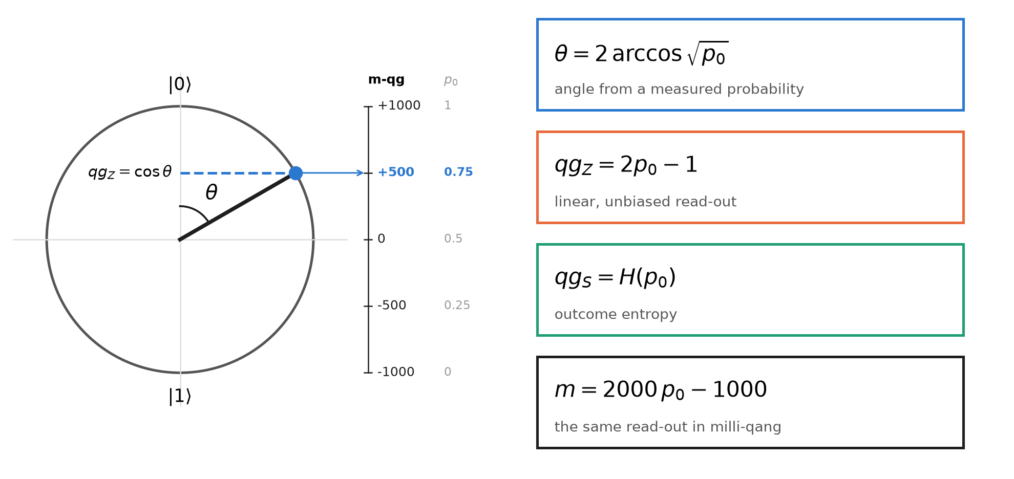
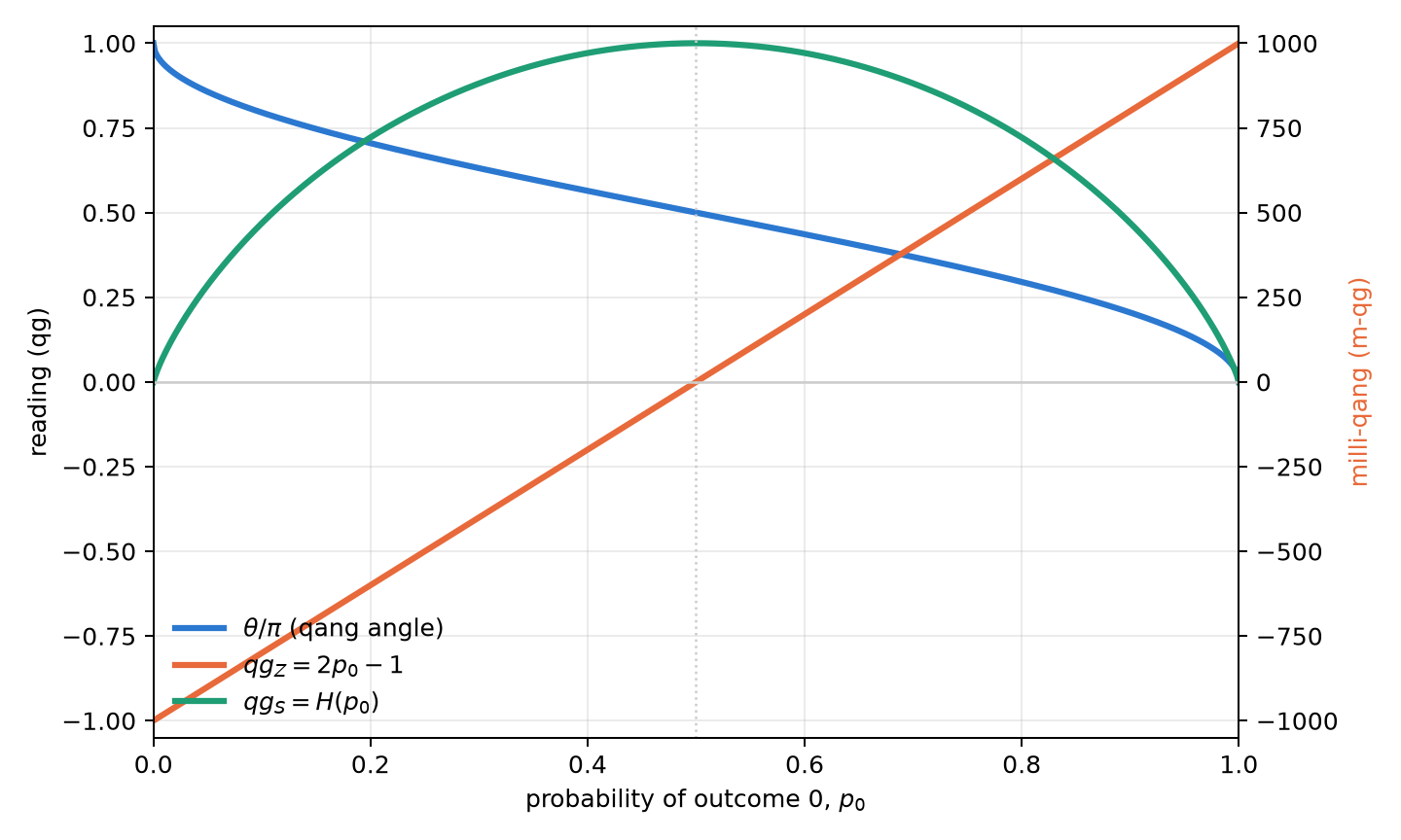
The other two readings of the unit come from the same probability: the qang angle \(\theta=\arccos(qg_Z)\in[0,\pi]\) and the superposition spread \(qg_S=H(p_0)\in[0,1]\), the Shannon entropy of the outcome (studied below). Figure 1.1 summarizes the definition: the point on the circle is the state, its projection on the vertical axis is \(qg_Z\), and the scale on the right gives the same reading in milli-qang and in probability.
Three properties make \(qg_Z\) a good working coordinate:
- It is a bijection. On \(\theta\in[0,\pi]\), \(\cos\theta\) is strictly decreasing and covers \([-1,1]\): each value of \(qg_Z\) corresponds to a single latitude of the sphere.
- It is directly measurable. \(\widehat{qg}_Z = (n_0-n_1)/N\) is the average of the \(\pm1\) outcomes of the shots; it needs no inversion and no fit.
- It holds for any state. For a mixed state, \(qg_Z = \operatorname{Tr}(\rho\,\sigma_z)\), which reduces to \(\cos\theta\) when \(\rho=|\psi\rangle\langle\psi|\) (§3).
The sign and range have an immediate physical reading: \(qg_Z=+1\) is the pole \(|0\rangle\), \(qg_Z=-1\) the pole \(|1\rangle\), and \(qg_Z=0\) any point of the equator, where the measurement outcome is maximally uncertain.
An engineering unit. A useful unit does not need to be a new physical quantity; it needs to make what is measured legible. The decibel adds no physics to power: it expresses it on a scale that makes the gains of a chain of amplifiers additive. The qang plays an analogous role for the qubit: it expresses its state on the scale in which the experiment delivers it, so that preparation, noise and read-out are compared in the same units. It is an operational convention, and like every convention it is worth what it simplifies.
1.2 Theory of the milli-qang
1.2.1 Definition and scale
The deviations that matter in a real qubit are small: calibration errors, drift, read-out noise. A submultiple is convenient to express them, the milli-qang (m-qg):
\[ 1\ \text{qg} = 1000\ \text{m-qg},\qquad m = 1000\,qg_Z\ \in[-1000,\,+1000]\ \text{m-qg}. \]
The scale runs from \(-1000\) m-qg at the pole \(|1\rangle\) to \(+1000\) m-qg at the pole \(|0\rangle\), with zero on the equator. A state with \(qg_Z=0.5018\) sits at \(501.8\) m-qg; its difference from the ideal \(0.5\) is \(1.8\) m-qg. The same definition holds for the other axes, \(qg_X\) and \(qg_Y\), so the whole Bloch vector can be expressed in m-qg.
1.2.2 Linear in probability, not linear in angle
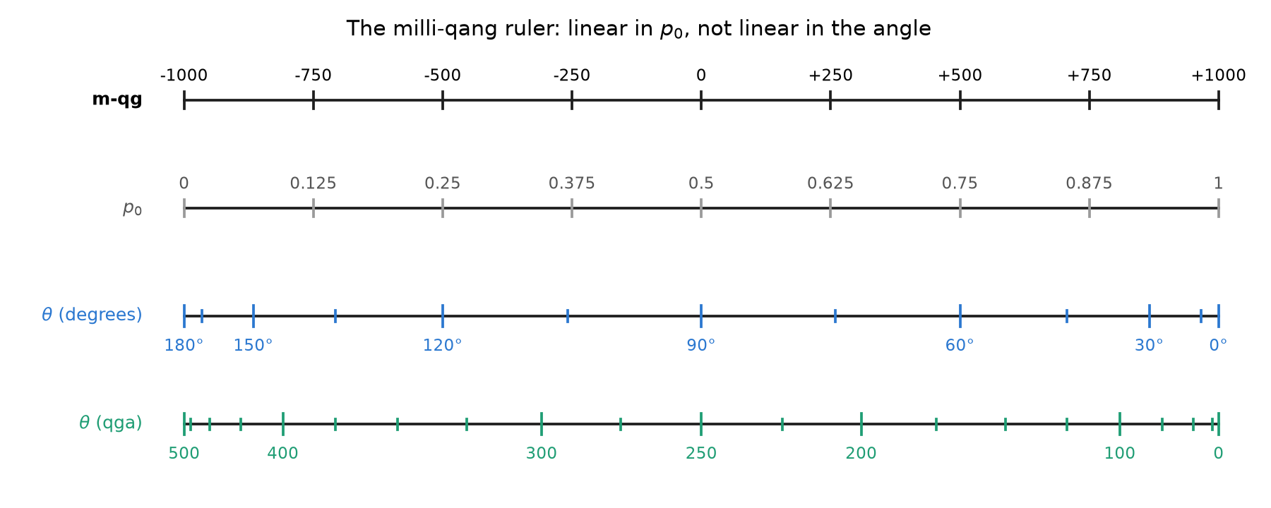
Since \(qg_Z=2p_0-1\), the milli-qang is linear in probability: one m-qg is always \(\Delta p_0=0.0005\), that is, 0.05 percentage points, anywhere on the scale. It is not linear in angle:
\[ \frac{dm}{d\theta} = -1000\,\sin\theta \qquad\Longrightarrow\qquad \Delta\theta \approx \frac{1}{1000\,\sin\theta}\ \text{rad per m-qg}. \]
On the equator (\(\theta=90^\circ\)) one m-qg is exactly one milliradian; at \(\theta=30^\circ\) it is two. Near a pole the linear relation fails and the exact one must be used: a state \(\delta\) m-qg below the pole \(|0\rangle\) makes with it the angle
\[ \theta_\delta = \arccos\!\left(1-\frac{\delta}{1000}\right)\approx\sqrt{\frac{2\delta}{1000}} . \]
One m-qg from the pole is \(0.0447\) rad (\(2.56^\circ\)); ten m-qg, \(8.1^\circ\). Figure 1.2 shows the consequence: on the milli-qang ruler the probability marks are evenly spaced and the angle marks crowd at the poles. That is why the unit is defined on probability and not on angle: it is the scale in which the instrument delivers the data.
1.2.3 Resolution from shots
With \(N\) shots, \(\widehat{qg}_Z\) has variance \(\sin^2\theta/N\) (derived in the arcsine section), so the standard deviation of the reading in milli-qang is
\[ \sigma_m = \frac{1000\,\sin\theta}{\sqrt N}\ \text{m-qg}, \qquad N_\delta = \left(\frac{1000\,\sin\theta}{\delta}\right)^{2} \]
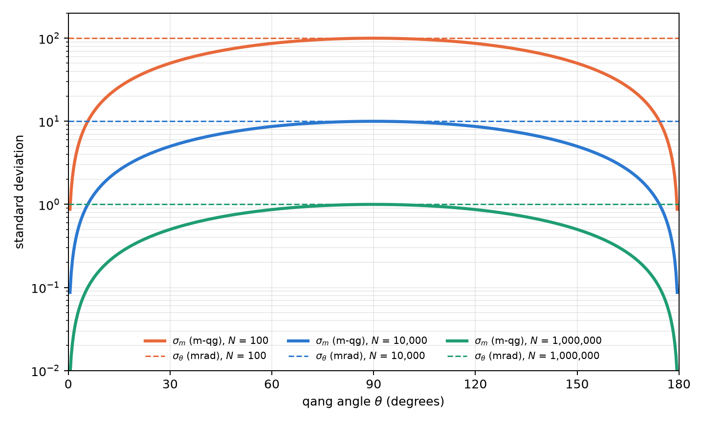
where \(N_\delta\) is the number of shots needed to resolve \(\delta\) m-qg at one sigma. On the equator, resolving 10 m-qg takes \(10^4\) shots and resolving 1 m-qg, \(10^6\). At \(60^\circ\) and 1000 shots, \(\sigma_m=27.4\) m-qg; to get down to 5 m-qg at that point takes 30,000 shots. Figure 1.3 compares \(\sigma_m\) with the uncertainty of the angle, \(\sigma_\theta=1/\sqrt N\): the m-qg reading is more precise near the poles, and the angle’s is the same all around the circle. The two curves touch on the equator, where one m-qg is one milliradian.
1.2.4 Gate error budget
The scale lets a gate error be expressed in the same units as the read-out. If the amplitude of a pulse has a random relative error of standard deviation \(\sigma\), the expected polar bias after \(R_x(\theta)\) is
\[ \mathbb E[qg_Z] = \cos\theta\; e^{-\theta^2\sigma^2/2} \qquad\Longrightarrow\qquad \varepsilon_m = 1000\cos\theta\left(e^{-\theta^2\sigma^2/2}-1\right)\ \text{m-qg} \]
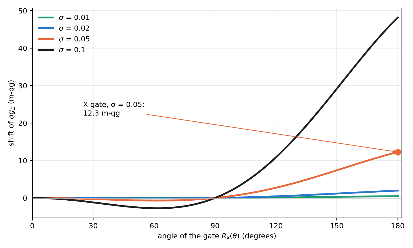
(§160). The error pulls the reading towards the equator: with \(\sigma=0.05\), an \(X\) gate (\(\theta=\pi\)) delivers \(qg_Z=-0.988\) instead of \(-1\), a shift of \(12.3\) m-qg. At multiples of \(\pi\) the shift grows with the square of the angle, always towards the equator; in general it goes as \(\theta^2\cos\theta\) (Figure 1.4). A \(\pi/2\) rotation does not shift at all, because it already sits on the equator. Chapter 2 uses this formula to choose, among equivalent representations of the same gate, the one with the smallest pulse area.
Chapters 2 and 3 use two derivatives of the reading with respect to the angle, which are worth naming here. The polar gradient and the curvature (or pulse impedance) are
\[ \nabla_{qg} = \frac{dm}{d\theta} = -1000\,\sin\theta\ \ \text{m-qg/rad}, \qquad \kappa_{qg} = \left|\frac{d^2m}{d\theta^2}\right| = 1000\,\lvert\cos\theta\rvert\ \ \text{m-qg/rad}^2 . \]
They are not new readings: they are derivatives of \(m=1000\cos\theta\). The curvature explains the budget above: to second order in the error, \(\lvert\varepsilon_m\rvert\approx\tfrac12\,\theta^2\sigma^2\,\kappa_{qg}\), so a random amplitude error shifts the reading in proportion to \(\kappa_{qg}\), which is 1000 at the poles and 0 at the equator.
1.3 The probability equation of the qang and the milli-qang
The previous sections lead to a single statement, which is the foundation of the whole book: every qang reading of a qubit is an exact function of a single probability, \(p_0\):
\[ \boxed{\; \theta = 2\arccos\sqrt{p_0},\qquad qg_Z = 2p_0-1,\qquad qg_S = H(p_0),\qquad m = 2000\,p_0-1000\ \text{m-qg} \;} \]
and, in the other direction, the probability equation of the milli-qang:
\[ p_0 = \frac{1000+m}{2000},\qquad \theta = \arccos\frac{m}{1000}. \]
There are no approximations: they are four readings of one number. Figure 1.5 shows them together. \(qg_Z\) and the milli-qang are the same straight line on two scales; the angle is monotonic but steepens at the poles; the entropy rises up to the equator and falls again, which is why it needs a branch to be inverted. Table 1.1 gives the reference values.
| \(\theta\) | \(p_0\) | \(qg_Z\) | m-qg | state |
|---|---|---|---|---|
| \(0\) | \(1\) | \(+1\) | \(+1000\) | pole \(\vert{}0\rangle\) |
| \(\pi/4\) | \(0.854\) | \(+0.707\) | \(+707\) | |
| \(\pi/3\) | \(0.75\) | \(+0.5\) | \(+500\) | |
| \(\pi/2\) | \(0.5\) | \(0\) | \(0\) | equator (\(\vert{}+\rangle\), \(\vert{}{+i}\rangle\), …) |
| \(2\pi/3\) | \(0.25\) | \(-0.5\) | \(-500\) | |
| \(\pi\) | \(0\) | \(-1\) | \(-1000\) | pole \(\vert{}1\rangle\) |
1.3.1 More than two outcomes: the statistical distance
The equation generalizes to a measurement with several outcomes. For two distributions \(p=(p_k)\) and \(q=(q_k)\), Wootters’ statistical distance (1981), or Bhattacharyya angle (Bhattacharyya 1943), is
\[ d(p,q) = \arccos\sum_k\sqrt{p_k\,q_k}. \]
For two outcomes, the distance between \((p_0,1-p_0)\) and the pole \((1,0)\) is \(\arccos\sqrt{p_0}=\theta/2\): up to the factor 2, the qang angle is the statistical distance between what is measured and the reference state. With three outcomes, for example, \(p=(0.5, 0.3, 0.2)\) and \(q=(0.4, 0.4, 0.2)\) are \(0.113\) rad apart. This is the door through which the unit leaves the qubit: Part II uses it for the Fisher information and the Fubini–Study metric, and the same geometry holds for any measured proportion, quantum or not.
1.4 The angular scale: the angular qang (qga)
The Geometric and Dimensional Foundation of the Qang System (Monteverde 2026a) proposes measuring angles on a thousand-based scale: one full turn is 1000 units. The book adopts that scale under another name, because throughout the book, the library and the chapters that follow, m-qg names the reading \(m=1000\,qg_Z\), which is linear in the probability and is not an angle (previous section). The angular scale is written qga (angular qang) and its thousandth m-qga:
\[ 1\ \text{turn} = 2\pi\ \text{rad} = 1000\ \text{qga} = 10^6\ \text{m-qga}, \qquad \theta[\text{rad}] = \frac{2\pi}{1000}\,\theta_{qga}, \qquad 1\ \text{m-qga}\approx 6.283\cdot10^{-6}\ \text{rad}. \]
With the Bloch polar angle in qga, the Born rule and the reading become
\[ p_0 = \cos^2\!\frac{\pi\,\theta_{qga}}{1000} = \frac{1+\cos(2\pi\theta_{qga}/1000)}{2}, \qquad m = 1000\cos\frac{2\pi\,\theta_{qga}}{1000}\ \text{m-qg}. \]
The pole \(\vert0\rangle\) is at 0 qga, the equator at 250 qga and the pole \(\vert1\rangle\) at 500 qga; the phase \(\varphi\) runs over \([0,1000)\) qga. The two scales complement each other: qga is uniform in the angle and m-qg is uniform in the probability. The state of Figure 1.1, for instance, sits at \(166.667\) qga and reads \(+500\) m-qg; at the equator, one m-qg of reading equals one milliradian, that is, \(0.159\) qga (\(159\) m-qga).
In code, since version 0.14.0, qang.qga does these conversions: p0_from_qga(250) gives 0.5, milliqang_from_qga(1000/6) gives +500 m-qg and qga_from_milliqang(-1000) gives 500 qga.
The azimuthal coordinate. The phase is read from two transverse measurements, \(\varphi=\operatorname{atan2}(qg_Y,\,qg_X)\), because \(qg_X=\sin\theta\cos\varphi\) and \(qg_Y=\sin\theta\sin\varphi\) and the ratio cancels \(\sin\theta\). As a fraction of a turn, \(qg_\varphi=(\varphi\bmod 2\pi)/2\pi\in[0,1)\) is exactly the azimuthal angle in qga divided by 1000. It is undefined at the poles, where \(qg_X=qg_Y=0\).
Geometry. The Fubini–Study metric of a qubit and the Fisher information of the \(Z\) measurement carry a constant factor in qga:
\[ ds^2 = \tfrac14\left(d\theta^2+\sin^2\theta\,d\varphi^2\right) = \frac{\pi^2}{10^6}\left(d\theta_{qga}^2+\sin^2\theta\,d\varphi_{qga}^2\right), \qquad I_F(\theta) = 1\ \text{rad}^{-2} = 4\pi^2\cdot10^{-6}\ \text{qga}^{-2}. \]
The second is the stabilization of the arcsine section in another unit: the standard deviation of the qang angle is \(159.15/\sqrt N\) qga over the whole circle (\(5.03\) qga with 1000 shots). The Berry curvature, \(F=\tfrac12\sin\theta\,d\theta\wedge d\varphi\), integrated over the sphere (\(\theta\) spans 500 qga and \(\varphi\) 1000) gives \(2\pi\), that is, Chern number 1.
Corrections to the Foundation. Three claims of the source document are not adopted, because its own formulas contradict them:
- It assigns \(p_0=0.5\) to 125 qga. Its own equation gives \(p_0(125\ \text{qga})=\cos^2(\pi/8)=0.854\) (+707 m-qg); \(p_0=0.5\) belongs to 250 qga.
- It gives curvature \(K=1\) to the metric \(ds^2=\tfrac14\,d\theta^2\). That metric, with its azimuthal term, is the one of a sphere of radius \(1/2\), whose Gaussian curvature is \(K=4\); \(K=1\) belongs to the Bloch sphere of radius 1.
- It suggests that a lattice in m-qga avoids barren plateaus. Changing the unit of the parameter multiplies every derivative by the constant \(2\pi/1000\): it changes neither the ratio of gradient variance to its scale nor its decay with the number of qubits. The unit has no effect on plateaus. The qang tools are another matter: they do mitigate them in tested regimes, namely the qg local cost (Section 23.7) and the weight filter under T1 (Section 20.6).
1.4.1 Unverified proposal: energy and antimatter in qga
The Foundation extends the scale to relativistic kinematics. What follows is an unverified proposal: the identities are corrected, but the physical reading is unproven and the rest of the book does not use it.
Relativistic angle. Dividing \(E^2=(mc^2)^2+(pc)^2\) by \(E^2\) gives \(\cos\theta_r=mc^2/E=1/\gamma\) and \(\sin\theta_r=pc/E=\beta\). The identity is exact, because \(1/\gamma^2+\beta^2=1\). With \(\theta_r\) in qga, \(E=mc^2/\cos(2\pi\theta_{r,qga}/1000)\): rest is at 0 qga and the ultra-relativistic limit (\(E=pc\)) at 250 qga. The angle \(\theta_r\) is tied to the rapidity \(\eta\) by \(\cos\theta_r=1/\cosh\eta\) (the Gudermann function), with no Wick rotation needed.
Antimatter. The Dirac equation has two branches, \(E_\pm=\pm\sqrt{(pc)^2+(mc^2)^2}=\pm\,mc^2/\cos\theta_r\). The Foundation assigns the negative branch a shift of 500 qga, tied to CPT symmetry; that identification has no support and is not adopted.
Probabilities. The Foundation equates \(P_\text{rest}=(mc^2/E)^2\) with \(p_0(\theta_{qga})\). There is a factor 2 in the angle: \((mc^2/E)^2=\cos^2\theta_r\), whereas \(p_0=\cos^2(\theta/2)\), so the equality holds only if the Bloch angle is \(2\theta_r\). If instead the Bloch angle is taken equal to \(\theta_r\), there is a known result behind the document’s formulas \(\cos^2(\pi\,\text{qg}/1000)\) and \(\sin^2(\pi\,\text{qg}/1000)\): in the free Dirac spinor the large component weighs \((E+mc^2)/2E=\cos^2(\theta_r/2)\) and the small one \(\sin^2(\theta_r/2)\). But those weights are not probabilities of “matter” and “antimatter”, as the source document calls them: both belong to the same positive-energy solution.
Appendix G (Appendix G) develops this proposal. It finds an exact reading of \(E=mc^2\), the expectation value of the Dirac matrix \(\beta\), which equals \(mc^2/E\) and is therefore a \(qg_Z\). It also shows that charge conjugation inverts that reading.
Proposed names. Table 1.2 lists the names the Foundation introduces and how the book treats them.
| Foundation name | definition | treatment in the book |
|---|---|---|
| relativistic angle \(\theta_r\) | \(\cos\theta_r=mc^2/E\), \(\sin\theta_r=\beta\) | exact identity; in qga, a proposal |
| \(E(\text{qg})=mc^2/\cos(2\pi\,\text{qg}/1000)\) | total energy as a function of \(\theta_r\) | exact, with \(\theta_r\) in qga |
| \(E_\pm\), matter and antimatter sheets | \(\pm\,mc^2/\cos\theta_r\) | Dirac branches; the 500 qga CPT shift is not adopted |
| \(P_\text{rest}\), \(P_\text{kinetic}\) | \((mc^2/E)^2\), \(\beta^2\) | they add to 1; they are not \(p_0\), \(p_1\) of the same angle (factor 2) |
| \(P_\text{matter}\), \(P_\text{antimatter}\) | \(\cos^2\), \(\sin^2\) of the half angle | weights of the spinor’s large and small components, not antimatter probabilities |
| Q-Hertz (qHz) | qga per second | unit of angular frequency; a proposal |
| Q-Fisher (qFi) | Fisher information per qga² | \(4\pi^2\cdot10^{-6}\) qga\(^{-2}\) for a pure qubit |
| Q-Shannon (\(qg_S\)) | Shannon entropy of the outcome | it is \(qg_S\); it is not the von Neumann entropy |
| Q-Curvature, Q-SNR, Q-Geodesic, dissipative deficit | \(qg_\kappa\), \(qg_{SNR}\), \(qg_L\), \(qg_\tau\) | defined and checked in Section 1.11 |
| Q-Force, Q-Conductance, Q-Momentum | phase gradient, qga per volt, \((\pi/500)\hbar\) | proposed names, not used in the book |
1.5 Why measure in qg: the geometry–probability gap
The relation \(p_0=\cos^2(\theta/2)\) between the control parameter and the observed quantity is non-linear, and its derivative vanishes at the poles. This has concrete consequences. If a variational algorithm wants to adjust the state according to what it measures, the chain rule introduces the factor
\[ \frac{dE}{dq} = -\frac{1}{\sin\theta}\,\frac{dE}{d\theta}, \]
which diverges at \(\theta=0\) and \(\theta=\pi\) (research notes, §1). And if \(\theta\) is to be estimated from \(N\) shots, the variance of \(\hat p_0\) changes with the state, so the uncertainty of each reading depends on where the qubit is (§5). Neither problem is exotic: both appear as soon as one reasons in terms of what the experiment delivers, and the probability equation is the tool to handle them.
1.6 Inversion and the branch sign
The angle is recovered with \(\theta=\arccos(qg_Z)\). The inversion has a limit: \(\cos\theta\) is even, so \(qg_Z\) does not distinguish \(\theta\) from \(-\theta\). As long as one works on \([0,\pi]\) there is no problem, but an optimizer that needs to cross a pole gets stuck. The remedy is to measure the sign of the sine as well: the pair \((qg_Z, s)\) with \(s=\operatorname{sign}(qg_X)\) is one-to-one on the whole circle (§65). In the H₂ molecule the variational optimum is at \(\theta\approx-0.22\); every update that uses only \(qg_Z\) stops at the Hartree–Fock state, while the signed version reaches the exact energy.
1.7 The outcome entropy: \(qg_S\)
The polar bias says where the qubit points; it does not say how unpredictable the measurement is. That is the role of the superposition spread, the Shannon entropy of the outcome:
\[ qg_S = H(p_0) = -p_0\log_2 p_0 - (1-p_0)\log_2(1-p_0) \in [0,1]. \]
Since \(qg_Z\) and \(qg_S\) depend on the same population \(p_0\), they are tied by an exact, branch-free identity (§7):
\[ qg_S = H\!\left(\frac{1+qg_Z}{2}\right), \]
valid for every single-qubit state, pure or mixed, however it was prepared. Its derivative, \(\tfrac{d\,qg_S}{d\,qg_Z}=\tfrac12\log_2\tfrac{1-qg_Z}{1+qg_Z}\), diverges at the poles: it is the entropic counterpart of the gradient singularity. Near a pole, a minimal change of the bias produces an enormous relative change of the entropy.
1.8 Invertibility of \(qg_S\) and its error bars
Unlike \(qg_Z\), the entropy is not invertible over the whole domain: \(qg_S(\theta)=qg_S(\pi-\theta)\). The population \(p_0\) decreases from 1 to 0 on \([0,\pi]\) and \(H\) rises up to \(p=\tfrac12\) and then falls, so \(qg_S\) is strictly increasing on \([0,\pi/2]\) and strictly decreasing on \([\pi/2,\pi]\) (Figure 1.5). Inversion requires choosing one of the two halves (§2).
Estimating \(qg_S\) from finite shots raises a further problem: the entropy is flat at its maximum, and the delta method gives a zero standard error exactly where \(qg_S\approx1\). The native qang solution is to build the Wilson interval for \(qg_Z\) and map it through the identity above; since \(H\) is unimodal, the image is a valid interval. Over 2000 repetitions that interval kept a coverage of 0.90–0.99 in every case tested, even where the Wald interval or the bootstrap fell below 0.40 (§51).
1.9 The qang angle as the arcsine transformation
The central statistical property of the unit follows from propagating shot noise. With \(\widehat{qg}_Z = 2\hat p_0-1\),
\[ \operatorname{Var}(\widehat{qg}_Z)=\frac{\sin^2\theta}{N}, \qquad \operatorname{Var}(\hat\theta)\approx \operatorname{Var}(\widehat{qg}_Z)\left(\frac{d\theta}{d\,qg_Z}\right)^2 =\frac{\sin^2\theta}{N}\cdot\frac{1}{\sin^2\theta}=\frac1N . \]
The \(\sin^2\theta\) factors cancel exactly: the uncertainty of the qang angle does not depend on the state (§5), which is the horizontal dashed line of Figure 1.3. It is not a coincidence. Since \(p_0=\cos^2(\theta/2)\), the qang angle is, up to the reflection \(\theta\to\pi-\theta\), the classical arcsine transformation of a proportion, \(\phi=2\arcsin\sqrt p\), introduced by Bartlett (1947), Anscombe (1948) and Freeman and Tukey (1950) precisely to stabilize the variance (§125).
The claim was checked with exact binomial sums, without simulation: with \(n=100\), \((n+\tfrac12)\operatorname{Var} (\hat\theta)\) lies between 1.000 and 1.001; the coverage of the interval \(\hat\theta\pm z/\sqrt{n+1/2}\) stays between 0.930 and 0.962 for \(n\in\{30,100,1000\}\). The prediction failed in one case, and it is worth saying: with \(np\approx2.5\) both the angular and the Wald intervals lose coverage. The stabilization is asymptotic, and the regime of very few events requires the exact intervals of chapter 4.
1.10 Mixed states and multi-qubit registers
The definitions extend unchanged to mixed states and to registers:
- Mixed states. \(qg_Z=\operatorname{Tr}(\rho\sigma_z)\) no longer determines the state. The classical mixture of \(|0\rangle\) with weight 0.2 and \(|1\rangle\) with weight 0.8 has \(qg_Z=-0.6\) and von Neumann entropy 0.72, a combination no pure state reproduces (§3). The qang angle \(\theta=\arccos qg_Z\) is still a function of \(p_0\), so it keeps \(\operatorname{Var}(\hat\theta)=1/N\) here too: the probability does not know whether the state is pure. What loses the stabilization is the estimate of the Bloch polar angle, \(\arccos(qg_Z/r)\), of a qubit of length \(r<1\): \(\operatorname{Var}=\big[1+\tfrac{1-r^2}{r^2\sin^2\theta}\big]/N\), equal to the quantum Cramér–Rao bound \(1/(Nr^2)\) on the equator (§45).
- Registers. Each qubit has its local profile, obtained by partial trace, and the register has a joint entropy normalized by the number of qubits (§4). The Bell state illustrates it: each qubit has \(qg_Z=0\) and a local entropy of 1 bit, but the normalized joint Shannon entropy of the outcomes is 0.5 (the von Neumann entropy of the register is 0). The register is globally pure and locally mixed; the local profiles are not enough to describe it, and chapter 5 returns to this point with the Bloch radius.
1.11 Derived quantities of the reading
The treatise’s formulation (Monteverde 2026a) names, on top of this base, seven derived quantities. All of them come from the reading —from \(qg_Z\), or from the full qg vector when needed—, so they add no information to \(p_0\): they name combinations that the rest of the book uses. Table 1.3 collects them with their definition, what they are in the usual terms of statistics or physics, and how they are treated here. Appendix H (Appendix H) catalogues these and the book’s other sub-measures with the decision each one improves and its evidence.
| quantity | definition | what it is | treatment in the book |
|---|---|---|---|
| Q-Hertz (qHz) | qga per second | angular frequency on the qga scale: 1 qHz \(=2\pi/1000\) rad/s | unit of convenience |
| Q-Fisher (qFi) | Fisher information per qga² | \(I_F=4\pi^2\cdot10^{-6}\) qga\(^{-2}\) about the qang angle, for every state | exact (Section 1.4) |
| Q-Shannon (\(qg_S\)) | \(H(p_0)=H\big((1+qg_Z)/2\big)\) | Shannon entropy of the outcome | exact (Section 1.7) |
| Q-Curvature (\(qg_\kappa\)) | \(-d^2qg_S/d\,qg_Z^2=1/[\ln2\,(1-qg_Z^2)]\) | Fisher information about \(qg_Z\), in bits | exact; in optimizers, no gain (Section 30.4) |
| Q-SNR (\(qg_{SNR}\)) | \(\lvert qg_Z\rvert/\sqrt{1-qg_Z^2}=\lvert\cot\theta\rvert\) | signal-to-noise of one shot | exact; sets the shots needed to read a sign |
| Q-Geodesic (\(qg_L\)) | \(\arccos\big(\sqrt{p_0p_0'}+\sqrt{p_1p_1'}\big)=\lvert\theta-\theta'\rvert/2\) | Bhattacharyya angle between two readings | exact; it is the Fubini–Study distance on a common meridian |
| Dissipative deficit (\(qg_\tau\)) | \(\sqrt{1-r^2}=\sqrt{1-qg_X^2-qg_Y^2-qg_Z^2}\) | \(2\sqrt{\det\rho}\), the lack of purity | exact; measures loss of purity of any origin |
The first three have already appeared. On the Q-Fisher, one precision: the formulation describes its constancy as that of a flat manifold, and it is not one. What is constant is the information about a single coordinate, the polar angle; the Bloch sphere with the Fubini–Study metric has Gaussian curvature 4 (Section 1.4).
Information curvature. Differentiating twice the identity \(qg_S=H((1+qg_Z)/2)\) of Section 1.7,
\[ \frac{d\,qg_S}{d\,qg_Z}=\frac12\log_2\frac{1-qg_Z}{1+qg_Z}, \qquad qg_\kappa=-\frac{d^2qg_S}{d\,qg_Z^2}=\frac{1}{\ln 2\,(1-qg_Z^2)} . \]
The denominator is the variance of one shot, so \(qg_\kappa=I_F(qg_Z)/\ln 2\): the curvature of the entropy is the Fisher information that one shot carries about the polar bias, expressed in bits. It is \(1/\ln2=1.443\) on the equator and diverges at the poles, where the entropy is most sensitive. For a pure state, \(1-qg_Z^2=\sin^2\theta\) and \(qg_\kappa=1/(\ln2\,\sin^2\theta)\). Mind the notation: \(qg_\kappa\) is not the pulse curvature \(\kappa_{qg}=1000\,\lvert\cos\theta\rvert\) of Section 1.2. That one is the second derivative of the reading with respect to the angle; this one, that of the entropy with respect to the reading. The formulation proposes using \(qg_\kappa\) to damp an optimizer’s step near the poles. Scaling the step by the inverse Fisher information is the natural gradient (Amari 1998), and Chapter 30 measures it (Section 30.4): on the coordinate \(qg_Z\) that step is, to first order, gradient descent on \(\theta\), and it brings no speed-up of its own.
Signal-to-noise per shot. A shot is \(\pm1\), with mean \(qg_Z\) and standard deviation \(\sqrt{1-qg_Z^2}\), for any state, pure or mixed. Their ratio and the number of shots a sign requires are
\[ qg_{SNR}=\frac{\lvert qg_Z\rvert}{\sqrt{1-qg_Z^2}}=\lvert\cot\theta\rvert, \qquad N_\text{sign}=\left(\frac{z}{qg_{SNR}}\right)^{2}, \]
with \(\theta=\arccos qg_Z\), the qang angle. With \(N\) shots the signal-to-noise is \(\sqrt N\,qg_{SNR}\), and \(N_\text{sign}\) is the number of shots for the sign of \(qg_Z\) to stand \(z\) standard deviations from zero: it is the stopping criterion the formulation proposes. At \(60^\circ\) (\(+500\) m-qg) \(qg_{SNR}=0.577\) and 27 shots are enough for a 3σ sign; at \(80^\circ\) it takes 290, and at \(89^\circ\), about 29 500. On the equator the signal vanishes and the criterion never ends. Like every formula of this chapter based on the normal approximation, it holds when \(N_\text{sign}\) is not too small; with few shots the exact binomial test is used.
Geodesic distance. Two readings \((p_0,p_1)\) and \((p_0',p_1')\) are at Wootters’ statistical distance of Section 1.3, and for two outcomes that distance is
\[ qg_L=\arccos\big(\sqrt{p_0p_0'}+\sqrt{p_1p_1'}\big)=\frac{\lvert\theta-\theta'\rvert}{2}, \]
because \(\sqrt{p_0p_0'}+\sqrt{p_1p_1'}=\cos\tfrac\theta2\cos\tfrac{\theta'}2+\sin\tfrac\theta2\sin\tfrac{\theta'}2 =\cos\tfrac{\theta-\theta'}{2}\). It is half the difference of qang angles, that is, the distance between readings on the scale that stabilizes the variance. If both states are pure and share the meridian, \(qg_L\) equals the Fubini–Study distance \(\arccos\lvert\langle\psi\vert\psi'\rangle\rvert\). With different azimuths it is a lower bound, because a measurement cannot tell two states apart better than their overlap does. Chapter 3 uses it between the states of a reflector (Section 3.4).
Dissipative deficit. The three readings \(qg_X\), \(qg_Y\) and \(qg_Z\) form the qg vector \(\mathbf r\), of length \(r\le1\), and
\[ qg_\tau=\sqrt{1-r^2}=2\sqrt{\det\rho}, \qquad \operatorname{Tr}\rho^2=1-\tfrac12\,qg_\tau^2 . \]
It is 0 for a pure state and 1 for the maximally mixed state. The 0.2/0.8 mixture of the previous section has \(r=0.6\) and \(qg_\tau=0.8\); each qubit of a Bell pair, \(qg_\tau=1\). The formulation associates it with \(T_1\) and \(T_2\) relaxation, which is one of its causes, but the quantity measures the loss of purity without telling its origin apart: an average over calibration errors produces it too (Chapter 2, Section 2.6). Unlike the previous ones, it is not a function of \(p_0\): it requires measuring in three bases.
1.12 Scope and limits of the base
It is worth stating precisely what this base brings and what it does not, before building the rest of the book on it.
What it is not. The qang unit is not new physics. The polar bias is the expectation value of \(\sigma_z\), the qang angle is the arcsine transformation of a proportion and the milli-qang is, mathematically, \(1000\,\langle\sigma_z\rangle\). None of these readings holds information that the probability \(p_0\) does not already have; the probability equation says so explicitly. Nor does it reduce the shots a given precision requires (Chapter 4).
What it is. A working scale, in the sense of the decibel: it puts preparation, gate error, shot noise and read-out in the same units, so that they add, compare and can be budgeted. The question that matters is then empirical: does reasoning in milli-qang predict what a real processor does?
First test on hardware (§168). It was answered with a pre-registered experiment on one qubit of IQM’s superconducting Garnet processor: 26 circuits of 4000 shots, with four predictions fixed before the run. The result was mixed, and it is reported in full:
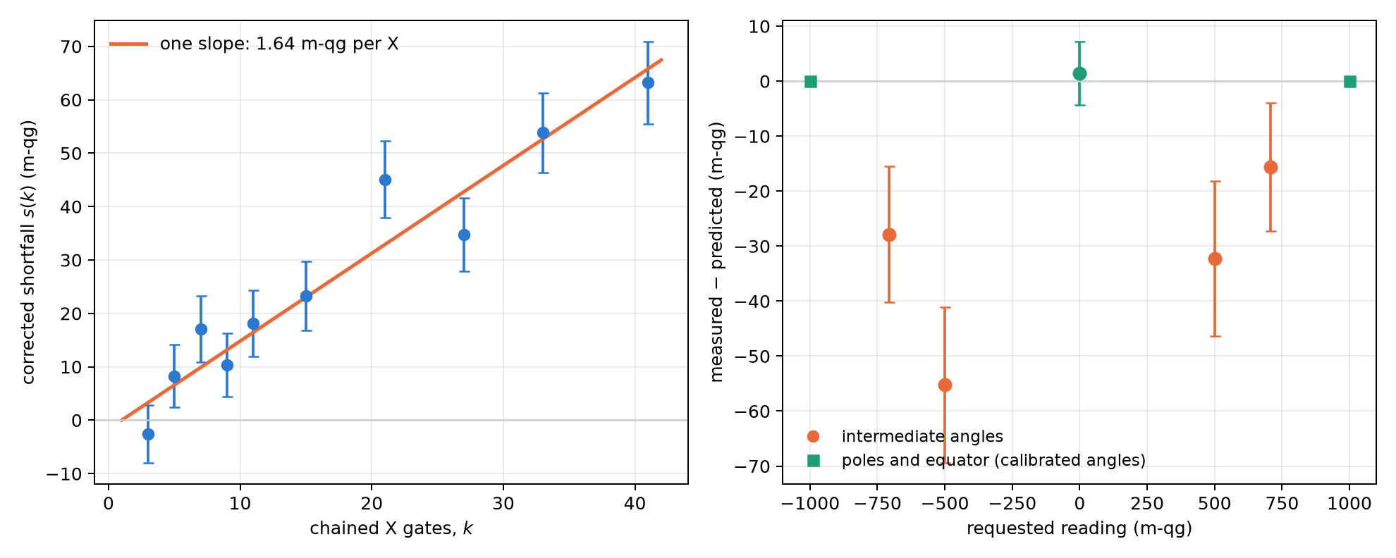
- The cost of a gate is measurable and budgetable in m-qg. Chaining 3 to 41 \(X\) gates, the shortfall of the reading (corrected for the readout errors measured at the poles) grows with a single slope: 1.64 m-qg per \(X\) gate, with a \(\chi^2\) per degree of freedom of 0.81. After 41 gates it is 63 m-qg, eight standard deviations above zero (Figure 1.6, left). Linear rather than quadratic growth points to incoherent error, relaxation during the pulses, and not to a coherent over-rotation.
- The scale makes visible an error that the readout model hides. The affine readout predicted from the poles fits at the equator, but the four intermediate angles read between 16 and 55 m-qg low (Figure 1.6, right). The processor calibrates the angles \(0\), \(\pi/2\) and \(\pi\) well; the others are over-rotated by \(1.3^\circ\) to \(3.9^\circ\). The prediction passed by the 4-of-5 rule, not cleanly.
- One prediction failed. The ten copies of the equator circuit scattered half as much as binomial shot noise allows, something independent shots cannot produce and which happens by chance with probability 0.013. A single run does not decide whether it was a fluke or a property of how the device returns batched circuits.
- Another prediction was badly designed. Fitting two parameters on four points left an extrapolation band so wide that any reading passed. It is recorded as a design flaw, not as a success.
The balance: on a real chip, the milli-qang turned the error of a gate into a budgetable number and exposed an angle error that the usual model does not see. But it was tested on one qubit, once, and shot noise did not describe the scatter of repeated circuits. Replication on more qubits and on another day is pending, and the book treats this base as solid mathematically and promising, but not yet consolidated, experimentally.
Second test on hardware (§170). On the same Garnet qubit, \(E=mc^2\) was read as a reading, with the \(\beta\) qubit of Appendix G (Section G.6). The Dirac eigenstate at \(0.6c\) read \(+759.9\pm14.9\) m-qg, where \(1000/\gamma=+800\) was predicted, and its mirror on the negative branch read \(-809.4\). The Zitterbewegung showed at the predicted frequency, 0.44% off. All five predictions passed. The low bias at intermediate angles appeared again, in the same direction as in §168, which points to a feature of the device rather than a fluke of one run. Both tests are on one qubit, and replication is still pending.
Open proposals. The author’s working version adds three proposals to this basis, which the book records as unverified:
- A regularized variational energy, \(E_\text{total}=\langle H\rangle+\lambda_\theta L_\text{qang}(\theta)+\lambda_\varphi L_\text{qang}(\varphi)\). Here the energy is the expectation value of a Hamiltonian, not the relativistic energy of the previous section. The form of the penalties \(L_\text{qang}\) and the values of the weights \(\lambda\) are not defined.
- A normalized radiation function, \(R(\theta,\varphi)=N\,[\,p_1+\alpha\cos\varphi\,]\), with the excited population \(p_1=\sin^2(\theta/2)\) as the emitting power. Neither \(N\) nor \(\alpha\) is fixed, and it is not checked against an emission model.
- Mechanisms against barren plateaus (local costs in m-qg, minimum-curvature \(\kappa_{qg}\) compilation, initialization with the branch sign). Two qang tools are already tested on the book’s networks. The qg local cost, \((1-\overline{qg_Z})/2\), the idea of Cerezo et al. (2021) written as a reading, has 470 times more gradient variance than the global cost with 10 qubits and shallow circuits (Section 23.7). The weight filter returns, under T1, exactly the noiseless gradient, to \(10^{-16}\), against a noise-induced plateau (Section 20.6; pre-registered prediction, §112). Both have measured limits: with deep circuits the local cost also decays exponentially and, where it escapes the plateau, it is classically simulable; and the weight sector itself flattens the gradient as the register grows, with or without the filter: like a polynomial at weight 1, which is simulable, and exponentially at half filling. Chapter 23 gathers the three sources of a plateau and what qang does with each (Section 23.8). Compilation by \(\kappa_{qg}\) and initialization with the branch sign have not been tested against plateaus.
1.13 Without qang and with qang
| action | without qang | with qang | difference |
|---|---|---|---|
| describe the outcome of a qubit | the probability \(p_0\) (or \(\langle Z\rangle\)) | \(qg_Z\), the angle \(\theta\), \(m\) and \(qg_S\), all exact functions of \(p_0\) | none in content: the same information; qang gives it a working scale from \(-1000\) to \(+1000\) |
| error bar of a reading | \(\sqrt{p_0(1-p_0)/N}\), different for each state | the angle has variance \(1/N\) for every state; in m-qg, \(1000\sin\theta/\sqrt N\) | convenience: the variance-stabilized coordinate of classical statistics (the arcsine) is the gate parameter |
| compare a gate error with shot noise | infidelity on one side, binomial deviation on the other, in different units | both in m-qg (on Garnet, 1.64 m-qg per \(X\) gate against the run’s shot noise) | in favour: one scale for the error budget |
| decide how many shots the sign of a reading needs | binomial test or normal approximation | \(N=(z/qg_{SNR})^2\), with \(qg_{SNR}=\lvert\cot\theta\rvert\) | convenience: it is the normal approximation written with the reading |
| express a gate or phase angle | radians, with factors of \(\pi\) | qga: 1000 per turn (\(X\) = 500 qga, equator = 250 qga) | convenience: the same information without factors of \(\pi\); it changes neither gradients nor plateaus |
| improve the device | — | — | none: the scale measures, it does not correct; prediction M2 of §168 failed |
Balance. The base adds no information to \(p_0\): it reorganizes it. What it gains is a uniform error bar in the angle and a common unit for gate errors and shot noise, which are exactly the two things the rest of the book uses.
1.14 In code
The qang.probability module is this chapter’s analysis tool: it reads counts and returns every reading, each with its interval.
import math
from qang import probability as pb

pb.readings_from_p0(0.75)        # theta = 1.047 (60°), qg_Z = 0.5, qg_S = 0.811, 500 m-qg

# 750 zeros in 1000 shots, against a target qg_Z = 0.5
r = pb.analyze(750, 1000, target_qg_z=0.5)
r.milliqang                      # (500.0, 444.5, 551.7) m-qg: estimate and Wilson interval
r.theta                          # (1.047, 0.986, 1.110) rad = 60.0°, 56.5°, 63.6°
r.qg_s                           # (0.811, 0.768, 0.852)
r.deviation_milliqang            # 0.0 m-qg from the target

pb.angle_per_milliqang(math.pi / 2)        # 0.001 rad: one m-qg is one milliradian on the equator
pb.pole_angle(1.0)                         # 0.0447 rad: one m-qg below the pole
pb.shots_for_resolution(10, math.pi / 2)   # 10000 shots to resolve 10 m-qg
pb.pulse_error_milliqang(math.pi, 0.05)    # 12.3 m-qg: X gate with a 5 % amplitude error
pb.statistical_angle([0.5, 0.3, 0.2], [0.4, 0.4, 0.2])   # 0.113 rad

# derived quantities
pb.quantum_snr(0.5)                        # 0.577: signal-to-noise of one shot at 60°
pb.shots_for_sign(0.5)                     # 27 shots for a 3σ sign
pb.information_curvature(0.0)              # 1.443 = 1/ln 2, the minimum curvature (equator)
pb.dissipative_deficit(0.0, 0.0, -0.6)     # 0.8: the 0.2/0.8 mixture
The figures of this chapter are generated by tools/make_cap01_figures.py, which uses the same functions.
1.15 Summary
- Definition. The polar bias \(qg_Z=\langle\sigma_z\rangle=2p_0-1=\cos\theta\) is bijective, directly measurable and valid for mixed states; the qang angle \(\theta=\arccos qg_Z\) and the entropy \(qg_S=H(p_0)\) complete the unit.
- Milli-qang. \(1\ \text{qg}=1000\) m-qg; the scale is linear in probability (1 m-qg \(=\Delta p_0=0.0005\)) and not linear in angle (1 mrad on the equator, \(2.56^\circ\) next to the pole). Resolving \(\delta\) m-qg takes \((1000\sin\theta/\delta)^2\) shots, and gate errors are budgeted in the same units.
- Probability equation. \(\theta\), \(qg_Z\), \(qg_S\) and \(m\) are exact functions of a single probability \(p_0\); with several outcomes, the qang angle generalizes to Wootters’ statistical distance.
- Angular scale. The angular qang measures angles with 1000 qga per turn and is distinct from m-qg, which is a reading: \(p_0=\cos^2(\pi\theta_{qga}/1000)\) and \(I_F=4\pi^2\cdot10^{-6}\) qga\(^{-2}\). The extension to relativistic energy and antimatter is an unverified proposal, with three errors of the source document corrected.
- Statistics. The qang angle is the arcsine transformation of a proportion: its variance is \(1/N\) for every state, pure or mixed; what needs a correction in a mixed state is the estimate of the Bloch angle.
- Derived quantities. \(qg_\kappa\) is the Fisher information about \(qg_Z\) in bits (and not the pulse curvature \(\kappa_{qg}\)); \(qg_{SNR}=\lvert\cot\theta\rvert\) sets the shots needed to read a sign; \(qg_L=\lvert\theta-\theta'\rvert/2\) is Wootters’ distance between two readings; \(qg_\tau=\sqrt{1-r^2}\) measures the lack of purity and is the only one that needs three bases.
- Scope. The unit is not new physics but a working scale. On real hardware (§168) it measured a cost of 1.64 m-qg per \(X\) gate, linear in the number of gates, and exposed reading shifts of 16–55 m-qg (over-rotations of \(1.3^\circ\)–\(3.9^\circ\)); a prediction about shot noise failed and replication is pending.
Bibliographic notes
The Born rule (Born 1926) and the Bloch sphere (Bloch 1946) are the starting point; for states, measurements and channels in general, see Nielsen and Chuang (2010). Wootters’ statistical distance (1981) and its relation to Fisher information are in Braunstein and Caves (1994); the Cramér–Rao bound, in Cramér (1946) and Rao (1945). The arcsine transformation that stabilizes the binomial variance comes from Bartlett (1947), Anscombe (1948) and Freeman and Tukey (1950), and the score interval is that of Wilson (1927). The binary entropy behind \(qg_S\) is that of Shannon (1948); the natural gradient, against which the information curvature \(qg_\kappa\) is compared, is that of Amari (1998). The numbered research notes (§) cited in this chapter and the scripts that check it are in the repository (Monteverde 2026b); the definition of the qang unit is in Monteverde (2026c). The angular qga scale and the relativistic proposal come from the working document Monteverde (2026a); the free Dirac spinor and its components are in any text on relativistic quantum mechanics.