3 Reflections, Householder and Grover dynamics
Grover’s algorithm is, at heart, a sequence of reflections. Written in qg units, each reflection is an algebraic matrix in the polar bias, the trajectory of the algorithm is a Chebyshev polynomial and the information each iteration brings has a closed form. Everything rests on the base of Chapter 1: the transition probability between two states is a probability like \(p_0\), with its own qang angle and m-qg reading, and the bias of Grover’s flag is read on the same scale. The derived quantities of Chapter 1 (Section 1.11) are read here on the algorithm: the geodesic distance \(qg_L\) between the states of a reflector, the signal-to-noise \(qg_{SNR}\) and the information curvature \(qg_\kappa\) along the trajectory, and the dissipative deficit \(qg_\tau\) as a measure of the visibility that noise leaves to amplitude estimation. The chapter develops that reading and sets it against what happens when the gates are noisy, where the qg reading loses to the simplest tool.
3.1 Transition matrices without transcendental functions
Chapter 2 showed that every single-qubit gate has the transition matrix
\[ T(q)=\begin{pmatrix}\tfrac{1+q}{2}&\tfrac{1-q}{2}\\[0.5ex]\tfrac{1-q}{2}&\tfrac{1+q}{2}\end{pmatrix}, \]
doubly stochastic and rational in \(q\). By construction it is unistochastic: it comes from a unitary. Its composition shows the difference between classical probability and quantum amplitude. Two classical channels with biases \(q_1\) and \(q_2\) compose by multiplication: \(T(q_1)T(q_2)=T(q_1q_2)\). Two successive quantum rotations instead give
\[ q_{12}=\cos(\theta_1+\theta_2)=q_1q_2-\sqrt{(1-q_1^2)(1-q_2^2)} . \]
The term \(-\sqrt{(1-q_1^2)(1-q_2^2)}\) is the interference: the transverse part of each state, invisible in \(T\), adding up in amplitude. With \(q_1=0.3\) and \(q_2=-0.5\), the classical composition gives \(-0.15\) and the quantum one \(-0.976\): in milli-qang, \(-150\) against \(-976\), an interference of 826 m-qg, close to half the scale. The transition matrix describes each gate on its own, but not the sequence: that needs the phases. On the angular qga scale of Chapter 1 (Section 1.4) quantum composition is simply additive: \(\theta_1=201.5\) qga, \(\theta_2=333.3\) qga, the sum is \(534.8\) qga and \(\cos(2\pi\cdot534.8/1000)=-0.976\). What is not additive is the reading in m-qg.
3.2 The Householder reflector in qg space
A reflection with respect to the state \(|\psi\rangle\) is the Householder operator \(I-2|\psi\rangle\langle\psi|\). For \(|\psi(q)\rangle=\sqrt{\tfrac{1+q}{2}}|0\rangle+\sqrt{\tfrac{1-q}{2}}|1\rangle\) it is
\[ H(q)=I-2|\psi(q)\rangle\langle\psi(q)|=-q\,\sigma_z-\sqrt{1-q^2}\;\sigma_x , \]
a Hermitian, unitary matrix with \(H(q)^2=I\), whose coefficients are the state’s own qg values: \(q\) on \(\sigma_z\) and its transverse part \(\sqrt{1-q^2}\) on \(\sigma_x\) (§166). On the Bloch sphere it is the rotation by \(\pi\) (500 qga) about the axis of the state, together with an overall sign change.
3.3 The Grover diffuser as a qg reflection
The Grover diffuser reflects about the initial state: \(D=2|\psi\rangle\langle\psi|-I\). Comparing with the previous section,
\[ D(q)=-H(q)=q\,\sigma_z+\sqrt{1-q^2}\;\sigma_x . \]
In the two-dimensional plane of the algorithm (the “good” state being searched for and the “bad” one, its complement), the oracle is the reflection about the bad axis and the diffuser the reflection about the initial state. The product of two reflections is a rotation by twice the angle between their axes: that is the whole of Grover’s dynamics. In the Fubini–Study metric (Section 1.4), each iteration covers the same arc length along a great circle: \(2t\) in Hilbert space, that is, \(4t\) in the Bloch angle of the flag qubit of the Chebyshev section.
3.4 Transition probability between qg states
The fidelity of two pure states is written with their qg vectors \(\mathbf r=(qg_X,qg_Y,qg_Z)\):
\[ |\langle\psi_1|\psi_2\rangle|^2=\frac{1+\mathbf r_1\cdot\mathbf r_2}{2}. \]
If the two states share a meridian (the same azimuthal phase), it depends on the polar biases alone:
\[ P(q_1\to q_2)=\frac{1+q_1q_2+\sqrt{(1-q_1^2)(1-q_2^2)}}{2}. \]
The condition matters: with different azimuths the polar biases are not enough and the full transverse part is needed. The formula was checked against the inner product on 200 random pairs (§166).
The transition probability in the equation of Chapter 1. \(P\) is a probability, so it has its own qang readings. If \(\gamma\) is the angle between the two Bloch vectors, \(\mathbf r_1\cdot\mathbf r_2=\cos\gamma\) and \(P=\cos^2(\gamma/2)\): it is Born’s rule with \(\gamma\) in place of \(\theta\). Therefore
\[ 2\arccos\sqrt P=\gamma,\qquad m_P = 2000\,P-1000 = 1000\;\mathbf r_1\cdot\mathbf r_2\ \text{m-qg}: \]
the qang angle of the transition probability is the angle between the states, and its milli-qang reading is a thousand times the dot product of their qg vectors. It is Chapter 1’s Wootters statistical distance applied to two states (Section 1.3). With \(q_1=0.3\) and \(q_2=-0.5\) on the same meridian, \(P=0.838\), \(m_P=+676\) m-qg and \(\gamma=0.828\) rad, which is exactly \(|\theta_1-\theta_2|=|\arccos 0.3-\arccos(-0.5)|\). In qga, \(\gamma=131.8\) qga and \(P=\cos^2(\pi\gamma_{qga}/1000)\).
The geodesic distance. The Fubini–Study distance between the two states, the shortest path between them over the state space, is
\[ qg_L=\arccos\sqrt P=\frac{\gamma}{2}, \]
the quantity \(qg_L\) of Chapter 1: in the example, \(0.414\) rad (\(65.9\) qga). On a common meridian it equals the Bhattacharyya angle of the two \(Z\) readings, so it is obtained from two single-qubit histograms without tomography. With different azimuths the \(Z\) reading underestimates it: two states with \(q=0.45\) and phases \(0\) and \(\pi\) have the same reading, and hence a zero Bhattacharyya angle in \(Z\), but \(\lvert\langle\psi_1\vert\psi_2\rangle\rvert=0.45\) and they are \(qg_L=\arccos0.45=1.104\) rad (\(175.7\) qga) apart. The full transverse part is then needed.
3.5 The Grover trajectory as a Chebyshev polynomial
Let \(a=\sin^2 t\) be the fraction of good states, read with a flag qubit whose initial bias is \(qg_0=1-2a=\cos 2t\). Each iteration advances the amplitude angle by \(2t\), so after \(k\) iterations the angle is \((2k+1)t\) and
\[ qg_k=\cos\big((2k+1)\,2t\big)=T_{2k+1}(qg_0), \]
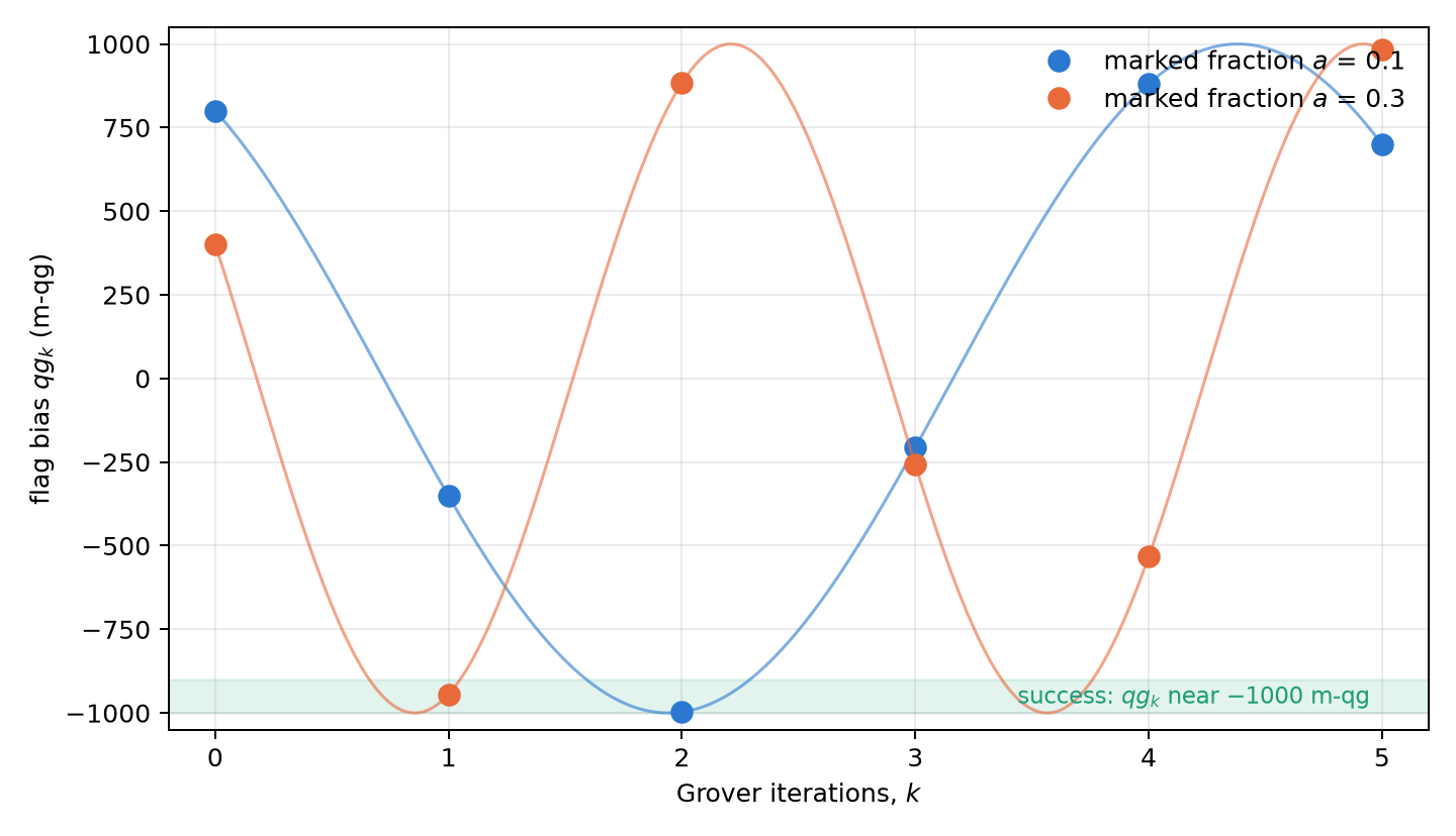
with \(T_m\) the Chebyshev polynomial of the first kind, \(T_m(\cos x)=\cos mx\) (§37). By the probability equation, the success probability is \(P_k=(1-qg_k)/2\), and certain success is the pole at \(-1000\) m-qg. For instance, with \(a=0.1\), \(qg_0=0.8\) and the successive iterations give \(+800\), \(-352\), \(-997\) and \(-206\) m-qg: the bias crosses the pole at \(k=2\) (\(P_2=0.9986\)) and then moves away (Figure 3.1). In qga the step is uniform: \(t=51.2\) qga, the flag’s Bloch angle starts at \(2t=102.4\) qga and advances \(4t=204.8\) qga per iteration; at \(k=2\) it reaches \(512.1\) qga, 12 qga past the pole (500 qga).
The Chebyshev structure yields for free the one-shot Fisher information at depth \(m=2k+1\). Since \(T_m'=mU_{m-1}\) and \(1-T_m^2=(1-q^2)U_{m-1}^2\),
\[ F_m=\frac{m^2}{1-qg_0^2}: \]
depth multiplies the qg information of Chapter 1 by \(m^2\), uniformly along the fringe. It is the qg form of the known factor \(4m^2\) for the angle (Suzuki et al. 2020). On the milli-qang scale, the resolution on \(qg_0\) with \(N\) shots at depth \(m\) is \(1000\sqrt{1-qg_0^2}/(m\sqrt N)\) m-qg: with \(a=0.1\) and 100 shots, 60 m-qg without iterating and 12 m-qg at depth \(m=5\). With respect to the flag’s initial angle, the information is \(m^2\) times that of Chapter 1 and does not depend on the state: \(m^2\cdot4\pi^2\cdot10^{-6}\) qga\(^{-2}\), with a resolution of \(159.15/(m\sqrt N)\) qga, that is, 15.9 qga without iterating and 3.2 qga at depth 5. In terms of the searched fraction, \(1-qg_0^2=4a(1-a)\), so \(F_m=m^2/[4a(1-a)]\) and the resolution is \(2000\sqrt{a(1-a)}/(m\sqrt N)\) m-qg.
3.5.1 The trajectory as a harmonic oscillation
The treatise’s formulation reads \(qg_k=\cos\big((2k+1)\,2t\big)\) as a sampled harmonic oscillator: the flag runs along a cosine at a constant angular step, \(4t\) per iteration. If each iteration lasts \(\Delta t\), that is an angular frequency of \(4t_{qga}/\Delta t\) qga per second, that is, in qHz (Section 1.11); with \(a=0.1\), 204.8 qga per iteration. The picture has a useful consequence. At the pole the cosine is at its turning point, where the velocity \(d\,qg/dk\) vanishes: there the success is insensitive, to first order, to an angle error. If the flag ends \(\delta\) away from the pole, \(P=\cos^2(\delta/2)\approx1-\delta^2/4\). The 12.1 qga of excess at \(k=2\) cost only 0.14 % of success (\(P_2=0.9986\)); 25 qga would cost 0.6 %, and 50 qga, 2.4 %. That is why the rounding of \(k^\ast\) matters little when \(a\) is small and a lot when the step is coarse. The geodesic distance to the solution says it in one figure: after \(k=2\), \(qg_L(qg_2,-1)=6.04\) qga, half the excess of Bloch angle.
The outcome entropy runs through the same cycle: \(qg_S\) is \(0.469\), \(0.909\), \(0.016\) and \(0.969\) bits at \(k=0,\dots,3\). It falls almost to zero at the optimum and rises again past it. Like the other derived quantities, it is a function of \(qg_k\) and cannot tell on which side of the pole the flag is.
Matter and antimatter: what the analogy allows. The treatise proposes reading the Grover rotation as a conversion channel between matter and antimatter, with the equator as a “neutral meson” and the inversion as charge conjugation. As a physical claim it is not adopted: the marked and unmarked subspaces of a search are not particle and antiparticle. What is exact is more modest. The oscillation of a neutral meson between its particle and antiparticle states is also a two-level rotation, and its mixing asymmetry \((N_\text{unmixed}-N_\text{mixed})/(N_\text{unmixed}+N_\text{mixed})=\cos(\Delta m\,t)\), valid when the two widths are equal (Navas et al. 2024), is a \(qg_Z\): it has qang angle \(\Delta m\,t\) and a uniform error bar in that angle, like any reading of Chapter 1. Grover and the meson share the kinematics, a cosine, and nothing else: the meson also decays. Appendix G (Appendix G) gives the correct reading of charge conjugation, which flips the expectation value of the Dirac matrix \(\beta\).
Two orthogonal states, such as the marked one and its complement, are \(qg_L=\pi/2\) apart, that is, 250 qga, the maximum distance; an ideal unitary evolution preserves purity (\(qg_\tau=0\)) along the whole arc.
3.6 Analytic limits: coarse angles and overshoot
The optimal number of iterations is \(k^\ast=\operatorname{round}\!\big(\tfrac{\pi}{4t}-\tfrac12\big)\); with \(t\) in qga, \(k^\ast=\operatorname{round}(125/t_{qga}-\tfrac12)\). When the searched fraction \(a=M/N\) is small, \(t\) is small, \(k^\ast\approx\tfrac{\pi}{4}\sqrt{N/M}\) and the rounding hardly matters. When \(M/N\) is not negligible, the angle per iteration is coarse: the bias jumps in large steps along the curve \(\cos((2k+1)2t)\) and can overshoot the pole. Iterating more does not help; it hurts, because the rotation keeps going. The qg reading makes this behaviour visible: \(qg_k\) samples a cosine at odd points. With \(a=0.3\), \(k^\ast=1\) gives \(-944\) m-qg (\(P=0.972\)) and one more iteration jumps to \(+884\) m-qg (\(P=0.058\)), the orange curve of Figure 3.1.
3.6.1 Signal-to-noise and curvature along the trajectory
The formulation proposes reading the trajectory with two derived quantities of Chapter 1: the per-shot signal-to-noise \(qg_{SNR}=\lvert qg_k\rvert/\sqrt{1-qg_k^2}\) and the information curvature \(qg_\kappa=1/[\ln2\,(1-qg_k^2)]\). Table 3.1 gives them for \(a=0.1\).
| iteration \(k\) | depth \(m\) | \(qg_k\) (m-qg) | Bloch angle (qga) | success \(P_k\) | \(qg_{SNR}\) | \(qg_\kappa\) |
|---|---|---|---|---|---|---|
| 0 | 1 | \(+800.0\) | \(102.4\) | \(0.1000\) | \(1.33\) | \(4.01\) |
| 1 | 3 | \(-352.0\) | \(307.2\) | \(0.6760\) | \(0.38\) | \(1.65\) |
| 2 (optimum) | 5 | \(-997.1\) | \(512.1\) | \(0.9986\) | \(13.15\) | \(250.8\) |
| 3 (overshoot) | 7 | \(-206.4\) | \(716.9\) | \(0.6032\) | \(0.21\) | \(1.51\) |
Near the pole both shoot up, and the formulation proposes using them as a pole-proximity detector to stop the iterations before the overshoot. Two precisions. First, they are functions of \(qg_k\): a threshold on \(qg_{SNR}\) or on \(qg_\kappa\) is a threshold on \(\lvert qg_k\rvert\), and it cannot tell whether the flag reached the pole or already passed it. At \(k=2\) it is 12 qga beyond the pole, and both take the same values as 12 qga before. What says whether another iteration pays is the formula for \(k^\ast\), not the quantity. Second, reading them costs shots: measuring the flag destroys the state, so every \(k\) queried is a separate run. The use they do bring is that of Chapter 1: \(qg_{SNR}\) says how many shots are needed to confirm the sign of the final reading, \(N=(3/qg_{SNR})^2\), that is, one shot at \(k=2\) and 64 at \(k=1\).
3.6.2 Grover with noise
With noisy gates the picture changes, and it is worth recording as it came out (§63). In searches on 4 to 6 qubits, with each multi-controlled Z compiled to 14, 36 and 84 CNOTs and depolarizing noise on every CNOT:
- Noise moves the best iteration earlier and eats the speed-up. With \(n=6\) and \(p_2=0.005\) the best iteration drops from 4 to 1 and the cost per verified success rises from 6.1 to 27.6 oracle calls, against 32 for classical search.
- The qg formula fails under gate noise. If the unmarked outcomes were uniform, each qubit would have \(qg_{Z,i}=\pm(NP-1)/(N-1)\), and the signs would give the answer and the magnitude the success probability without knowing it. Depolarizing noise is not uniform after the diffuser, and the label-free estimate was worse than the frequency of the most common outcome in every case.
- Reading the answer from signs loses. With \(n=5\), 100 shots find the marked item 66% of the time with the qg signs and 91% with the most frequent bitstring.
The honest balance: in Grover search the outcome histogram is a better estimator than the per-qubit qg reading. qg provides the Chebyshev picture and the information factor, not a better estimator. The author’s working version further proposes a regularized variational energy for reflection circuits and a radiation function that would follow \(P_k\) during amplification; these are the open proposals of Chapter 1 (Section 1.12), unverified.
3.7 Amplitude estimation
Where the Chebyshev structure does pay off is in amplitude estimation: using increasing depths to estimate \(a\) with fewer oracle queries than direct sampling. With maximum-likelihood estimation (depths 0, 1, 2, 4, …, 100 shots each), without noise, the error falls as queries\(^{-0.93\ldots-1.12}\) against queries\(^{-0.5}\) for Monte Carlo, and is 8.4–9.3 times lower at 26 200 queries (§37).
Noise sets limits. With depolarization \(p=0.01\) per iteration, a likelihood that ignores the noise ends worse than Monte Carlo (\(6.8\cdot10^{-3}\) against \(2.7\cdot10^{-3}\)), while one that includes it keeps a 4× advantage. With \(p=0.05\), not even the noise-aware likelihood beats Monte Carlo: beyond a depth of order \(1/p\) the iterations carry almost no signal.
The dissipative deficit of Chapter 1 places that limit on the qg scale. In the visibility model of the likelihood, every iteration shortens the flag’s qg vector by a factor \(V\); after \(k\) iterations the fringe has amplitude \(V^k\) and
\[ qg_\tau=\sqrt{1-V^{2k}} . \]
With \(V=1-p\), \(V^k\approx e^{-kp}\): towards \(k\approx1/p\) the fringe falls to \(1/e\) of its amplitude and \(qg_\tau\) exceeds \(0.93\), so further iterations add depth on an almost mixed state. With a visibility of \(0.975\) per iteration, the middle of the range fitted on IonQ (next paragraph), \(qg_\tau\) is \(0.63\) after 10 iterations and \(0.80\) after 20. It is the same \(1/p\) depth frontier, read as loss of purity.
On IonQ’s calibrated noisy simulator (3 qubits, \(a=0.3\), 36 000 queries), the estimate was accurate, with an RMS error of 0.0005–0.0015 and a fitted visibility of 0.965–0.985 per iteration, and 7 to 30 times better than a realistic Monte Carlo, whose depth-zero circuit is biased by the device noise (§39).
3.8 Without qang and with qang
| action | without qang | with qang | difference |
|---|---|---|---|
| transition probability between two states | \(\lvert\langle\psi\vert\phi\rangle\rvert^2\) | \((1+\mathbf r_1\cdot\mathbf r_2)/2\), with qang angle equal to the angle between the states and reading \(1000\,\mathbf r_1\cdot\mathbf r_2\) m-qg | none in value; qang makes it geometric |
| Grover trajectory | \(\sin^2((2k+1)\theta_0)\) | \(qg_k=T_{2k+1}(qg_0)\), success at \(-1000\) m-qg | equivalent; the Chebyshev form shows that the m-qg resolution improves by a factor \(m\) with depth |
| distance between two states | \(\arccos\lvert\langle\psi\vert\phi\rangle\rvert\) | \(qg_L=\gamma/2\), which on a common meridian comes from two \(Z\) histograms | convenience; with different azimuths the \(Z\) reading is not enough |
| decide when to stop iterating | \(k^\ast\) from the formula | threshold on \(qg_{SNR}\) or \(qg_\kappa\) | none: they are functions of \(\lvert qg_k\rvert\) and do not see whether the pole was passed; the formula for \(k^\ast\) does |
| read the search with noise | bit-string histogram | per-qubit qg reading | against: the qg reading loses to the histogram |
| estimate an amplitude with noise | maximum likelihood on counts | the same, with the noise written into the qg likelihood | in favour up to a depth near \(1/p\), not beyond |
Balance. The chapter’s identities are exact, but none gives a number that the usual amplitude does not. The only comparison with real noise in the chapter is unfavourable to the qg reading, and it is written down as such.
3.9 In code
from qang import algebra, probability

algebra.householder_qg(0.45)        # -0.45 Z - 0.893 X, a reflection: H @ H = I
algebra.grover_diffuser_qg(0.45)    # +0.45 Z + 0.893 X
P = algebra.transition_probability(0.3, -0.5)        # 0.838, same meridian
algebra.transition_probability(0.3, -0.5, 0.0, 1.2)  # different azimuths
probability.readings_from_p0(P)     # theta = 0.828 rad (the angle between the states), +676 m-qg
algebra.geodesic_distance(0.3, -0.5)                 # qg_L = 0.414 rad (65.9 qga) = gamma / 2

qg_2 = algebra.chebyshev_trajectory(0.8, 2)          # -0.9971 (-997 m-qg, P = 0.9986), a = 0.1
probability.quantum_snr(qg_2)                        # 13.15
probability.information_curvature(qg_2)              # 250.8
algebra.grover_fisher_information(0.8, 5)            # 69.4 per shot: 25 times that of m = 1
algebra.geodesic_distance(qg_2, -1.0)                # 0.038 rad (6.04 qga) from the solution
3.10 Summary
- The transition matrix of a gate is rational in \(q\), but it does not compose like the gate: the difference between \(q_1q_2\) and \(\cos(\theta_1+\theta_2)\) is the interference.
- The Householder reflector and the Grover diffuser are \(\mp(q\,\sigma_z+\sqrt{1-q^2}\,\sigma_x)\).
- The transition probability between two states is \((1+\mathbf r_1\cdot\mathbf r_2)/2\); on a common meridian it depends on the polar biases alone. Read with the equation of Chapter 1, its qang angle is the angle between the states and its reading is \(1000\,\mathbf r_1\cdot\mathbf r_2\) m-qg. The geodesic distance is \(qg_L=\gamma/2\).
- The Grover trajectory is \(qg_k=T_{2k+1}(qg_0)\), with certain success at \(-1000\) m-qg, and the Fisher information at depth \(m\) is \(m^2/(1-qg_0^2)\): the m-qg resolution improves by a factor \(m\).
- \(qg_{SNR}\) and \(qg_\kappa\) shoot up near the pole, but as a stopping criterion they do not see whether the flag has already passed it; what they bring is the number of shots to confirm the sign of the final reading.
- The trajectory is a sampled cosine: at the pole it is at its turning point, so an excess of 12 qga costs only 0.14 % of success. The matter–antimatter reading of the rotation is not adopted; what is exact is that a neutral meson’s mixing asymmetry, \(\cos(\Delta m\,t)\), is a \(qg_Z\).
- With noise, the per-qubit qg reading loses to the histogram in search; in amplitude estimation the advantage holds if the noise enters the likelihood, and ends near depth \(1/p\), where the flag’s dissipative deficit, \(qg_\tau=\sqrt{1-V^{2k}}\), exceeds \(0.93\).
Bibliographic notes
The reflector is that of Householder (1958). Grover search is Grover (1996), and amplitude amplification and estimation, Brassard et al. (2002); maximum-likelihood estimation without phase estimation is Suzuki et al. (2020). The transition probability between qg states is the distance of Wootters (1981). The numbered research notes (§) cited in this chapter and the scripts that check it are in the repository (Monteverde 2026a); the definition of the qang unit is in Monteverde (2026b).