14 Postselected closed timelike curves (P-CTC) and the resolution of paradoxes – Quantum Computing, Information and Physics in qang Space

14.1 From the base: the success probability has qang angle \(\varphi\)

In the simplest model the qubit that “travels to the past” undergoes a rotation \(R_X(\varphi)\), and the postselection succeeds with probability

\[ P_{\text{success}}=\cos^2\frac{\varphi}{2}. \]

It is the probability equation of Chapter 1 with \(p_0=P_{\text{success}}\), so its qang angle is exactly the rotation, \(\arccos(2P-1)=\varphi\), its reading is \(m=1000\cos\varphi\), and the success rate measured over \(N\) attempts gives \(\varphi\) with uncertainty \(1/\sqrt N\). The grandfather paradox, \(\varphi=\pi\), sits at the south pole: \(P=0\), \(m=-1000\).

14.2 Two ways to close a time loop

Deutsch (D-CTC, 1991). (Deutsch 1991) The system in the loop must be self-consistent: its state \(\rho_C\) is a fixed point of the evolution, \(\rho_C=\operatorname{Tr}_S[U(\rho_S\otimes\rho_C)U^\dagger]\). At least one fixed point always exists, so there is never a paradox, but there may be several, and an extra rule is needed to choose; the usual one takes the maximum-entropy fixed point.

Postselection (P-CTC; Bennett and Svetlichny, Lloyd and co-workers, 2011). (Svetlichny 2011; Lloyd et al. 2011) The qubit sent to the past, \(C\), is half of a Bell pair \((C,A)\). After \(C\) interacts with the system \(S\), \((C,A)\) is projected back onto the Bell state: it is a teleportation of \(C\) to its own past, with the Bell measurement forced to its trivial outcome. The effective evolution of \(S\) is

\[ \rho_S\mapsto\frac{\operatorname{Tr}_C(U)\,\rho_S\,\operatorname{Tr}_C(U)^\dagger}{\operatorname{Tr}[\ldots]}, \]

which is not linear because of the normalization. In the circuit the projection is a Bell measurement keeping the shots that read 00: a filter on the Bell sector.

14.3 The success law and the grandfather paradox

With \(R_X(\varphi)\) on \(C\) alone, \(\operatorname{Tr}_C(U)=\operatorname{Tr}R_X(\varphi)/2=\cos(\varphi/2)\), and the success is \(\cos^2(\varphi/2)\). At \(\varphi=\pi\) the qubit flips its own past: it is the grandfather paradox, and in P-CTC it has probability zero. It is not resolved: it does not happen. In D-CTC the same case has the maximally mixed state as its fixed point, and it happens with probability 1, like a coin.

On three simulated noise models, with 8000 shots (§164), the success law holds within 0.05 except at \(\varphi=0\) on two devices (C1 failed: 0.950 and 0.931 against 1), and the paradox is suppressed to the noise floor on two of three (C2 failed on FakeTorino):

Table 14.1: The P-CTC success law at the extremes, simulated noise models.

simulated device	success at \(\varphi=0\) (exact 1)	success at \(\varphi=\pi\), the paradox (exact 0)
FakeBrisbane	0.950	0.019
FakeTorino	0.931	0.056
FakeFez	0.983	0.009

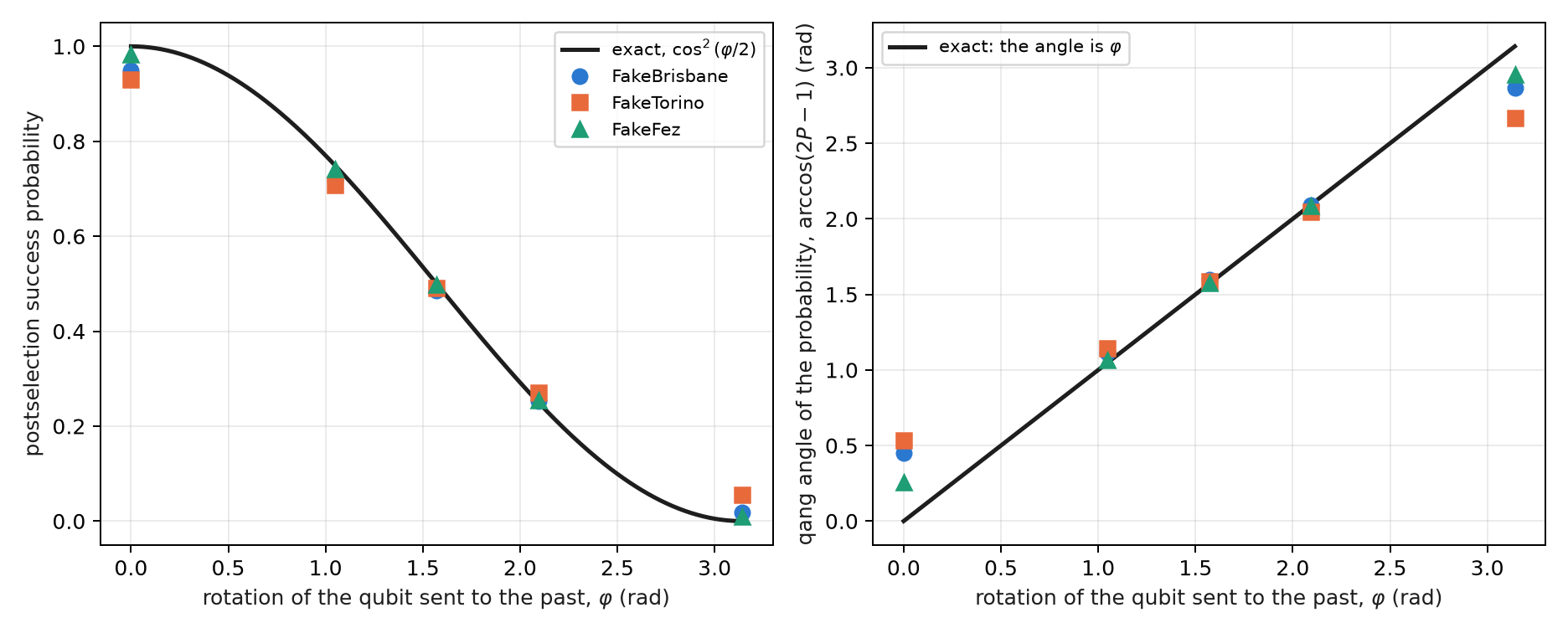
Figure 14.1: Left: postselection success probability against the rotation, exact and on three simulated noise models. Right: its qang angle, which is the rotation itself; the largest deviations are at the poles, where a small probability error is a large angle error.

Figure 14.1 shows something specific to the angle reading. In the interior, the qang angle of the measured rate reproduces \(\varphi\) to a few hundredths of a radian; at the poles it deviates by up to half a radian. It is the non-linearity of the milli-qang in angle from Chapter 1: next to the pole, 1 m-qg is 2.56°, and the devices’ 34–138 m-qg of error at \(\varphi=0\) become 0.26–0.53 rad, that is, 41.6–84.6 qga on the angular scale of Chapter 1 (Section 1.4). On that scale the success rate is \(\cos^2(\pi\varphi_{qga}/1000)\), and the grandfather paradox sits at \(\varphi=500\) qga.

14.4 The rotation controlled by the system

If it is the system \(S\) that controls the rotation of \(C\), the partial trace is an operator on \(S\):

\[ \operatorname{Tr}_C(U)=\operatorname{diag}\!\left(1,\ \cos\tfrac{\varphi}{2}\right), \]

and the branch of \(S\) that would produce the paradox is damped by \(c=\cos(\varphi/2)\). From \(|+\rangle\), the postselected state of \(S\) has

\[ qg_Z(S)=\frac{1-c^2}{1+c^2},\qquad qg_X(S)=\frac{2c}{1+c^2}, \]

with success \((1+c^2)/2\). At \(\varphi=\pi\), \(qg_Z(S)=1\): the system is forced into the branch that does not flip the past. On the simulated models FakeFez follows the curve within 0.061 over the whole range, FakeBrisbane reads 0.903 at \(\varphi=\pi\), and FakeTorino loses most of the suppression (0.600): prediction C3 failed.

14.5 What a qg reading tells apart between D-CTC and P-CTC

This section is new in the book: it is exact density-matrix algebra, computed in the figure script, with no device run. The same controlled circuit is taken, with \(S\) in \(|+\rangle\), and the output of \(S\) is computed in both formulations.

In D-CTC the channel on \(C\) is \(\rho_C\mapsto\tfrac12\rho_C+\tfrac12R_X\rho_CR_X^\dagger\), and every state that commutes with \(R_X(\varphi)\) is a fixed point. With the maximum-entropy rule, \(\rho_C=I/2\), and the output of \(S\) is

\[ qg_Z(S)=0,\qquad qg_X(S)=\cos\frac{\varphi}{2},\qquad r=\cos\frac{\varphi}{2}. \]

The two formulations separate in different readings (Figure 14.2):

Table 14.2: The system S after the controlled loop, in both formulations.

\(\varphi\)	P-CTC: \(m_Z\), \(m_X\) (m-qg)	D-CTC: \(m_Z\), \(m_X\) (m-qg)	P-CTC success
0	0, 1000	0, 1000	1
\(\pi/3\)	143, 990	0, 866	0.875
\(\pi/2\)	333, 943	0, 707	0.750
\(2\pi/3\)	600, 800	0, 500	0.625
\(\pi\)	1000, 0	0, 0	0.500

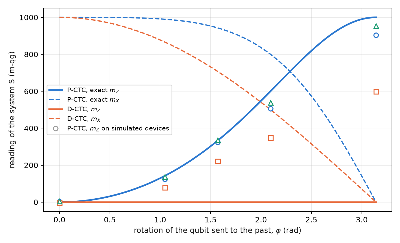
Figure 14.2: Readings of the system S after the controlled loop. P-CTC (blue) moves the population, \(m_Z\), toward the paradox-free branch; D-CTC (orange) leaves \(m_Z=0\) and only decoheres, lowering \(m_X\). The markers are the P-CTC on three simulated noise models.

The difference is qualitative. P-CTC changes the populations of \(S\) (the paradoxical branch loses weight) and leaves a pure state; D-CTC does not touch the populations and only removes coherence. A \(Z\) reading of \(S\) already decides between the two models, and the simulated devices, with all their noise, sit on the P-CTC side, as they must, because the circuit is the P-CTC one.

Deutsch’s ambiguity can be read too. At \(\varphi=\pi/2\) the state \(|+\rangle\) is also a fixed point, and it gives the same \(qg_Z(S)=0\) and the same \(qg_X(S)=0.707\), but \(qg_Y(S)=-0.707\) and radius 1, against \(qg_Y=0\) and radius 0.707 with \(I/2\). The two D-CTC solutions differ in the local radius of Chapter 5: the maximum-entropy rule picks the fixed point that leaves \(S\) most mixed.

14.6 The cost of postselection

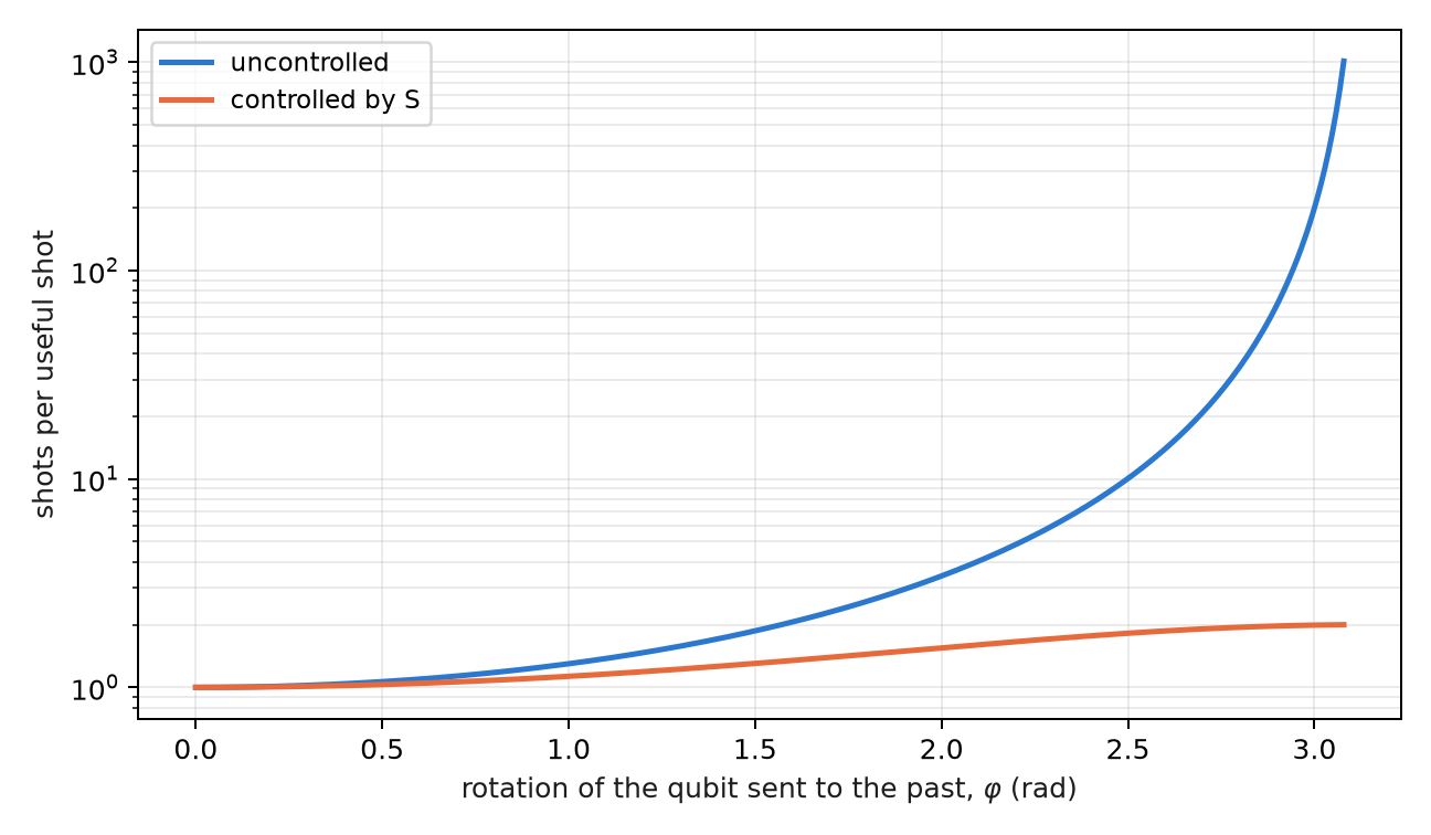
“Time travel” in this model costs shots. Each useful shot needs, on average, \(1/P_{\text{success}}\) shots: 2 at \(\varphi=\pi/2\), 4 at \(2\pi/3\), 400 at a tenth of a radian from the paradox (Figure 14.3). With the controlled rotation the cost never exceeds 2, because half of the superposition of \(S\) pays nothing. It is the same accounting as the sector filter of the previous chapters, with one difference: here the discarded fraction is not noise but the model’s physics, and it cannot be reduced.

Figure 14.3: Shots needed per useful postselected shot, uncontrolled and with the rotation controlled by S.

14.7 What remains open

Two topics of the index have no support yet and stay proposals: the non-linearity of P-CTCs applied to discriminating non-orthogonal states (the circuit and the prediction are missing), and a device run of the D-CTC against P-CTC comparison, which would require preparing Deutsch’s fixed point and not only postselecting.

14.8 Without qang and with qang

Table 14.3: The chapter’s actions without the qang scale and with it.

action	without qang	with qang	difference
read the loop’s rotation	invert \(\cos^2(\varphi/2)\)	the qang angle of the success rate is \(\varphi\), with \(\sigma=1/\sqrt N\)	equivalent in the interior; at the poles the angle reading amplifies the error (34–138 m-qg become 0.26–0.53 rad), which counts against
verify the suppression of the paradox	success probability and the state of S by tomography	\(m_Z(S)\): 903, 600 and 955 m-qg against 1000	unit; the suppression is the postselection’s
tell D-CTC from P-CTC	compare density matrices	P-CTC moves \(m_Z\); D-CTC does not and lowers \(m_X\)	in favour: a single \(Z\) reading decides the model
tell apart the D-CTC fixed points	entropy of each solution	the local radius of Chapter 5: 0.707 against 1	in favour: the ambiguity becomes a reading
reduce noise	—	the postselection is the filter; the qang scale adds nothing	none

Balance. In this chapter qang pays as a diagnostic tool: with one or two readings it says which loop model is operating and which of Deutsch’s solutions was chosen. The success law is the probability equation of Chapter 1, and with it come its limits next to the poles.

14.9 In code

import math
from qang import postselection as ps

ps.pctc_success(2 * math.pi / 3)                 # 0.25: postselection success
math.acos(2 * ps.pctc_success(2.0) - 1)          # 2.0: the qang angle is the rotation
ps.pctc_controlled_qg_z(math.pi)                 # 1.0: the paradoxical branch, suppressed
qc = ps.pctc_circuit(math.pi, controlled=True)   # S, C, A; success = C and A read 0

14.10 Summary

The time loops of this chapter are information models: teleportation with postselection on a Bell outcome.
In P-CTC the success probability is \(\cos^2(\varphi/2)\) and its qang angle is \(\varphi\); the grandfather paradox has probability zero and, on two of three simulated models, sits at the noise floor.
With the controlled rotation, \(qg_Z(S)=(1-c^2)/(1+c^2)\): the paradoxical branch is suppressed; FakeTorino loses most of the suppression.
D-CTC does not change the populations of S and only removes coherence; a \(Z\) reading separates the two models, and the local radius separates Deutsch’s fixed points.
Postselection costs \(1/P\) shots per useful shot; it is the model’s physics, not noise, and it cannot be reduced.

Bibliographic notes

The self-consistent model of closed timelike curves is Deutsch (1991); the postselection model and its experimental test, Lloyd et al. (2011), and the comparison between the two, Svetlichny (2011). The numbered research notes (§) cited in this chapter and the scripts that check it are in the repository (Monteverde 2026a); the definition of the qang unit is in Monteverde (2026b).